Benchmarking w-event differential privacy mechanisms
About
Providing strong privacy for sensitive data is a pivotal requirement for many applications. The current gold standard for ensuring privacy on streaming data is w-event differential privacy. It assures the commonly accepted differential privacy guarantee for each running window of at most w time stamps. Since its original introduction [1], various mechanisms are proposed implementing w-event DP. However, there are currently no established standards how to compare w-event mechanisms empirically. Thus, existing study results are hard to compare. The objective of this project is to establish ways of how to compare mechanisms. This shall foster future research as well as the application of w-event mechanisms in practice.
This website corresponds to the paper:
Schäler, Christine; Hütter, Thomas; Schäler, Martin: Benchmarking the utility of w-event differential privacy mechanisms: when baselines become mighty competitors. 2022, KIT scientific working papers no. 194. (link)
On this website you can:
- Download the the benchmark including all mechanism implementations as Java sources,
- download the Access download links for real-world streams used in other studies and learn about our data preprocessing,
- learn about how to integrate new mechanisms into our framework,
- get pointers to w-event DP literature
W-event Differential Privacy
Definition
The w-event differential privacy framework is the current gold standard for ensuring differential privacy of continuously computed queries over data streams. The key idea is not to protect the stream entirely, as this would require an infinite amount of noise. Instead, one protects every running window of at most w time stamps [1].
We implement mechanisms satisfying w-event differential privacy using independent differentially private sub-mechanisms, as long as the budget spend by these mechanisms does not exceed 𝜖 for every rolling window of size w [1].
Known Mechanisms
Baseline mechanisms Sample and Uniform
Sample and Uniform are baseline mechanisms in the original article proposing w-event DP [1]. Specifically, Sample releases a new query result only every wth time stamp using full budget 𝜖 for perturbation. At all remaining time stamps, Sample approximates the current query result with the last released one. Uniform releases a new query result at every time stamp using 𝜖 / w budget for perturbation at each time stamp.
BA and BD mechanism
BA and BD are sophisticated mechanisms from the original article proposing w-event DP [1].
AdaPub
The AdaPub mechanism is published in [2].
DSAT-W
The DSAT-W mechanism is published in [3].
FAST-W
The FAST-W mechanism is used as competitor in [1]. It is an adaption of FAST mechanisms for finite time series from [6].
PeGaSus
The PeGaSus mechanism is published in [5].
RescueDP
The RescueDP mechanism is published in [4].
Download
Source code and runnables
Sources at GitHub: (link)
Benchmark
The benchmark is a Java project allowing for easy comparison of w-event mechanism implementations. It consists of four parts: Data generator, mechanisms implementation, real-world data integration connector, and the experiment framework.
Data generator
To benchmark the effect of stream properties, like seasonality or domain, and to mitigate the issue of not (or not anymore) available real-world streams, the benchmark contains a data generator. The generator mimics seasonal one-dimensional streams. It is implemented in the data generator package. For understanding how to use it, have a look at the method Experiment.runArtificalExperiments(). There, you see that one first has to create a Generator object providing the desired length (i.e., number of timestamps) of the stream prefix to create. In addition, one needs to provide the desired average period length and the basis for the exponential growing function. The shrinking phase of each season is symmetric to the growing phase. Next, one creates an object of type StreamScalerAndStretcher s providing the Generator object and the number of streams to create. Then, s.get_stream(i, desired_max_value, 1) gives you the i'th stream, scaled to domain [0,desired_max_value]. The final arguments are used to stretch the period length. Thus, providing value 1 means one does not change the period length. The figure below shows exemplary output.
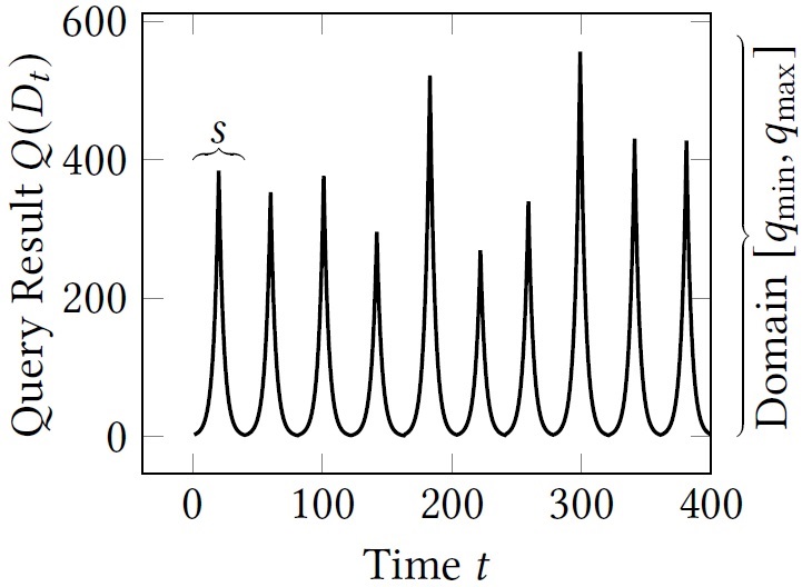
Example streams generated using our data generator with parameters t=400, domain [0,600] and expected season length of 40.
How to add a mechanisms?
Our benchmark contains implementations of all mechanisms stated above. Integrating a new mechanism is fairly simple. Each mechanism must extend the abstract mechanisms class. In addition, one needs to implement two abstract methods. The method name() simply returns the name of the mechanism used in all console outputs and result files. The more important method to implement is the run() method. The purpose of this method is to sanitize a streams prefix given as argument. The sanitized stream is the return value. The data format of the stream is ArrayList org_stream. That is, org_stream.get(0) returns the n-dimensional original query result of the first time stamp, org_stream.get(1) the original query result of the second time stamp. The query result of time stamp is double array, independent whether the query is one- or multidimensional. Please do not modify the org_stream, it is passed by reference to each benchmarked mechanism. To get an intuition on how such an implementation may look like, have a look at the implementation of the baseline mechanism Sample and Uniform. The implementation of Uniform is shown in the figure below. As you see, the mechanism uniformly distributes the available budget over all w time stamps. Note, the Mechanism class offers various methods, such as sanitizing a query result with the provided noise scale, you may deem helpful.
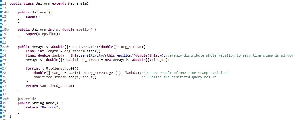
Implementation of mechanism Uniform.
Real-world data integration connector
To integrate new real-world streams, the integration connector helps you. For all streams considered in our paper, there is already respective code lading these (pre-processed data). Basically, we do not want to make any restriction how and where you store your data. Thus, integrating a new stream requires to change some lines of codes. There are three steps to do in the Experiment class. First, register your new stream by giving id (i.e., number) not assigned to any of the other streams. To this end, go to line 22 in the Experiment class and add Line like "public static final int MY_NEW_STREAM = 9;" In the current version, the first free id is 9. Next, go to Experiment.load(int) method. As you, see the id of the stream is used to call the right method really doing work. Add a new else if branch here. Finally, you need to implement method reading the input file and transforming it into our data format. A result is an ArraysList of double arrays. This is the input provided to the run() method of each mechanisms. Thus, the entries in the ArrayList are the time stamps. Instead, the values in the double array are the query result of corresponding dimension.
Experiment framework
Subject of the experiment framework is to run an experiment including multiple mechanisms either on a set of real-world streams or on a set of generated streams. For starting an experiment, simply call the main() method in the experiment.Experiment class. In case one sets runRealWoldExperiments = true, the systems runs experiments on real-world streams. Otherwise on artificially generated streams. Notable configuration options are:
- Mechansim.TRUNCATE: If enabled the sanitized query result q is post processed min(round(q),0), which significantly increases utility for sparse streams. For experiments on artificial data, we generally recommend to disable truncating.
- LaplaceStream.USAGE_MODE: There are three usage modes. For experiments, always use USAGE_MODE_RANDOM. The other two modes are for debugging only. For debugging USAGE_MODE_STUPID highly helps as one simply adds the expected error (i.e., lambda). That is mechanisms behavior becomes deterministic. The final usage mode USAGE_MODE_PRECOMPUTED uses a stream of pre-computed numbers following a Laplace distribution.
- Experiment.sensitivity: Currently, all queries re count queries with a global sensitivity of 1. Change this class member in case you want to do experiments with different sensitivity.
- Experiment.ERROR_MEASURE: The framework supports computing MAE or MRE as error measure.
Real-world streams
Next, we state where and how to download frequently used streams used for evaluating newly proposed w-event mechanisms. Note, for licensing reasons in most cases we must not publish a copy of the data. Thus, we also describe the pre-processing we conducted or recommend. Where meaningful, we directly post the python script conducting the preprocessing. In addition, we state notable features and insights regarding each stream we came across upon our own studies. Formally, most streams resemble the aggregated original query result (i.e., Q(S)) instead of the raw data S one would need to aggregate. So far, all Q(S) are multidimensional count queries with global sensitivity ΔQ = 1.
In case the download links are not available anymore or the data has been moved, do not hesitate to contact us: Contact.
Frequently used freely available streams
Flu Outpatient (link)
Stream counting the number of weekly outpatient count of the age group [5-24] from seasons 1997 to 2021. It contains a single dimension and about 1,200 time stamps. The stream features large seasonal changes having a domain in [0,10.000]. Hence, truncating the query result to positive integers results in no significant utility improvement.
To download data: mark "ILINet", "National"
Preprocessing
Use column with age group [5-24]. Preprocessing as in [7].
Flu Death (link)
Stream counting the number of flu deaths in the age group 18-64 of seasons 2012-2019. Older/more seasons are not available anymore -- note: AdaPub uses seasons 2009-2017. It contains a single dimension and about 400 time stamps. The stream features moderate seasonal changes having a domain in [0,350], with large number of small counts. Hence, truncating the query result to positive integers results in a significant utility improvement.
Preprocessing
Preprocessing as in [2].
Unemployment (link)
The streams contains the count of the monthly unemployment level of African American women of age group [16-19] from January 1972 to October 2011. It contains a single dimension with 478 time stamps. In contrast to the other streams, it features a level significantly s.t. the query domain is about [220,700]. Hence, truncating the query result to positive integers results in no utility improvement.
Preprocessing
Preprocessing as in [7].
State Flu (link)
Stream counting the number of infected persons in all 51 US states having an influenca-like illness. It contains 51 dimension and 492 time stamps. The stream features large seasonal changes having a domain in [0,10.000] with a moderate number of small counts. Hence, truncating the query result to positive integers results in some utility improvement.
To download data: mark "ILINet", "State"
Preprocessing
Preprocessing as in [2]:
df = pd.read_csv('../DataSets_struc/Health/ILINet.csv')
print(df)
transformed = df.pivot_table (index=['YEAR','WEEK'], columns='REGION',values='ILITOTAL',aggfunc=np.sum, fill_value=np.nan).dropna(axis=1)
print(transformed)
transformed.drop(columns=['Florida']) # contains only 'x'
print(transformed)
TDrive (link)
The original streams S contains taxi trajectories in Bejing of one-week trajectories of 10,357 taxis. Q(S) are location counts per grid cell. The stream contains 100 dimension and 672 time stamps. The query domain is [0,39,871] with moderate number of small counts. Hence, truncating the query result to positive integers results in some utility improvement.
Preprocessing as in [3].
The original stream consists of one week of data.
To allow for experiments with higher values of w, we extended the stream to four weeks.
We did this by duplicating the stream four times.
In addition, we cleared obvious outliers not being in the data set boundaries of  (116, 39.5) and (116.8, 40.3).
Retail - Appears to have been removed (08/2022)
The stream contains retail counts. It contains 4070 dimension and 374 time stamps. In accordance with AdaPub paper, we downsampled to 1289 dimension. The query domain is [0, 372306] with a moderate number of small counts. Hence, truncating the query result to positive integers results in some utility improvement.
Citation Request: Daqing Chen, Sai Liang Sain, and Kun Guo, Data mining for the online retail industry: A case study of RFM model-based customer segmentation using data mining, Journal of Database Marketing and Customer Strategy Management, Vol. 19, No. 3, pp. 197-208, 2012 (Published online before print: 27 August 2012. doi: 10.1057/dbm.2012.17).
Preprocessing as in [2].

import pandas as pd
import numpy as np
from datetime import datetime
# See PyCharm help at https://www.jetbrains.com/help/pycharm/

custom_date_parser = lambda x: datetime.strptime(x, "%d.%m.%Y %H:%M")
df = pd.read_csv

df = pd.read_csv('../retail.txt', date_parser=custom_date_parser, sep=";", parse_dates=['InvoiceDate'])
# get the number of customers per date per item
transformed = df[['InvoiceDate','StockCode','CustomerID']].pivot_table(index='InvoiceDate',  columns = 'StockCode', values='CustomerID',aggfunc='sum', fill_value=0)
# resample to days
resampled = transformed.resample('1D').sum()
#sample 1289 columns
resampled_1289cols = resampled.sample(n=1289, axis='columns',random_state=2)
# save as csv
resampled_1289cols.to_csv('AdaPub-OnlineRetail-l=374_d=1289')
World Cup - Appears to have been removed (08/2022)
The streams access counts of 89,997 URLs of the FIFA 1998 Soccer World Cup website and is the most frequently used benchmark data set. It contains 89,997 dimension and 1,320 time stamps. The stream has a query domain in [0,16,928], but is dominated by zero counts, i.e., it is very sparse.
Downsampled to 1289 dimensions as in [2], to be consistent with Retail stream.
Remaining preprocesing as in [1].
Taxi Porto (link)
The original streams S contains taxi drive trajectories in Porto and was used for ECML/PKDD 2015 competition. Q(S) are location counts per grid cell. The stream contains 1289 dimension (after downsampling) and 672 time stamps. The query domain is [0, 317] with a large number of small counts. Hence, truncating the query result to positive integers results in significant utility improvement.
Downsampled to 1289 dimensions, to be consistent with Retail stream.
Changed temporal resolution to 30s intervals to have the same length as TDrive stream.
Remaining preprocesing as in [8].
Exemplary results
In the figure below, each box contains the results w.r.t. both error metrics (L1 error and L2 error) for one experiment (vary-ϵ, vary-w). Each column shows the results of a one-dimensional real-world stream that we used in our benchmark. By comparing two sub-figures (i.e., rows) in a box, we see that 6 the raw L2 error approximately equals the square of the L1 error, which is expected. The result patterns, however, are mostly identical. In most cases, the best (worst) mechanism w.r.t. L1 error is also the best (worst) mechanism w.r.t. L2 error. The anomalies of RescueDP (better utility for lower ϵ) on the Unemployment stream are more prominent in the L2 error space rather than the L1 error space.
Abstractly speaking our results suggest that usually MEA and MRE, as well as L1 and L2 error show a similar result pattern. Thus, on does not need to test every combination.
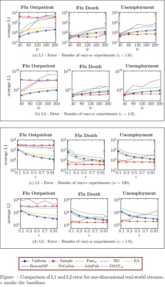
Exemplary results of L1 error and L2 error MAE metrics.
Bibliography
Literature regarding w-event DP. We include the original proposition of w-event DP, known mechanism, as well as tightly related literature.
[1] G. Kellaris et al. Differentially Private Event Sequences over Infinite Streams. Proc. VLDB Endow. 7, 12 (2014). [PDF]
Original Article proposing w-event DP and mechanisms Sample, Uniform, BA, and BD.
[2] T. Wang et al. Adaptive Differentially Private Data Stream Publishing in Spatio-temporal Monitoring of IoT. IPCCC (2019). [PDF]
Article proposing AdaPub mechanism and reference for preprocesing of various streams.
[3] H. Li et al. A Differentially private histogram publication for dynamic datasets: An adaptive sampling approach. CIKM (2015). [PDF]
Article proposing DSAT-W mechanism.
[4] Q. Wang et al. Real-time and spatio-temporal crowd-sourced social network data publishing with differential privacy. TDSC 15, 4 (2018). [PDF]
Article proposing RescueDP mechanism.
[5] Y. Chen et al. PeGaSus: Data-Adaptive Differentially Private Stream Processing. CCS (2017). [PDF]
Article proposing PeGaSuS mechanism. Note, the original implementation assures event-level DP only. We extended the guarantee to achieve w-event DP.
[6] L. Fan and L. Xiong. Real-time aggregate monitoring with differential privacy. CIKM (2012). [PDF]
Article proposing Fast mechanism for timeseries. Note, the original implementation assures user-level DP only. [1] extended the guarantee to achieve w-event DP.
[7] L. Fan and L. Xiong. An Adaptive Approach to Real-Time Aggregate Monitoring With Differential Privacy. TKDE 26, 9 (2014). [PDF]
Article describing preprocesing of Flu Outpatient and Unemployment stream.
[8] Q. Wang et al. RescueDP: Real-time spatio-temporal crowd-sourced data publishing with differential privacy. INFOCOM (2016). [PDF]
Article proposing RescueDP and describing preprocesing of Taxi Porto stream.